Software Versions:
ts_wep: v6.1.1
lsst_distrib: w_2023_19
Introduction
We perform a comparison between two strategies of averaging wavefront information encoded in the intensity of defocal point source images. The first approach, “pairing”, is to estimate wavefront based on pairs of intra and extra-focal donuts from each corner wavefront sensor. These individual wavefront estimates per donut pair can be aggregated into eg. mean, and thus conveyed to the optical feedback controller as a per-corner wavefront estimate. Another approach - “stacking” - is to stack donut images in each wavefront sensor before wavefront estimation, thus arriving at a single wavefront estimate from a “stacked” donut image. We compare these two approaches at providing a single wavefront estimate per sensor as a function of donut magnitude, and background.
Simulating a grid of stars
We make a grid of stars with code similar to ComCam rotation notebook and corner grid notebook
The transformation of pixel coordinates to focal plane radians is achieved with detector.getTransform(PIXELS, FIELD_ANGLE) (assuming (0,0) boresight). The same list of coordinates is used to retrieve the OPD.
The actual simulation is performed by running imgCloseLoop once with the artificial wfs_grid star catalog:
python /sdf/group/rubin/ncsa-home/home/scichris/aos/ts_phosim/bin.src/imgCloseLoop.py --inst lsst --numOfProc 180 --boresightDeg 0.0 0.0 --skyFile /sdf/data/rubin/u/scichris/WORK/AOS/DM-36218/wfs_grid.txt --output /sdf/data/rubin/u/scichris/WORK/AOS/DM-36218/wfs_grid/
The same was also run with quickbackground, achieved by substituting quickbackground for backgroundmode 0 in ts_phosim/policy/cmdFile/starDefault.cmd.
All simulations set the instrument as lsst (i.e. four corner wavefront sensors), and boresight as ra,dec=0,0. The table below summarizes the main variable parts of simulations: presence of sky background, and the magnitude of simulated stars. For details please consult the phosim background approximations chart.
phosim background mode |
stellar magnitude |
|---|---|
|
12,13,14,15,16,17 |
|
12,13,14,15,16,17 |
To be able to use the donuts detected at the zeroth iteration of imgCloseLoop, when simulating fainter sources the phosimData/lsstPipeline.yaml (created in each run of the AOS loop) was modified to increase the magnitude limit:
referenceSelector.magLimit.maximum: 18.5
Thus imgCloseLoop was run for fainter sources, but with the custom lsstPipelineIncreaseMagLimit.yaml config:
python /sdf/group/rubin/ncsa-home/home/scichris/aos/ts_phosim/bin.src/imgCloseLoop.py --inst lsst --numOfProc 180 --boresightDeg 0.0 0.0 --skyFile /sdf/data/rubin/u/scichris/WORK/AOS/DM-36218/wfs_grid.txt --output /sdf/data/rubin/u/scichris/WORK/AOS/DM-36218/wfs_grid/ --pipelineFile /sdf/data/rubin/u/scichris/WORK/AOS/DM-36218/lsstPipelineIncreaseMagLimit.yaml
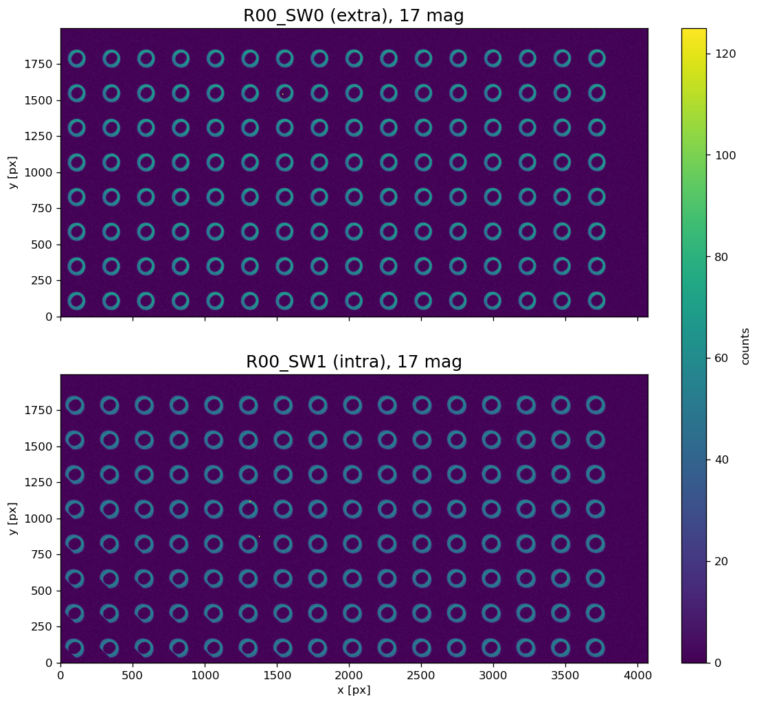
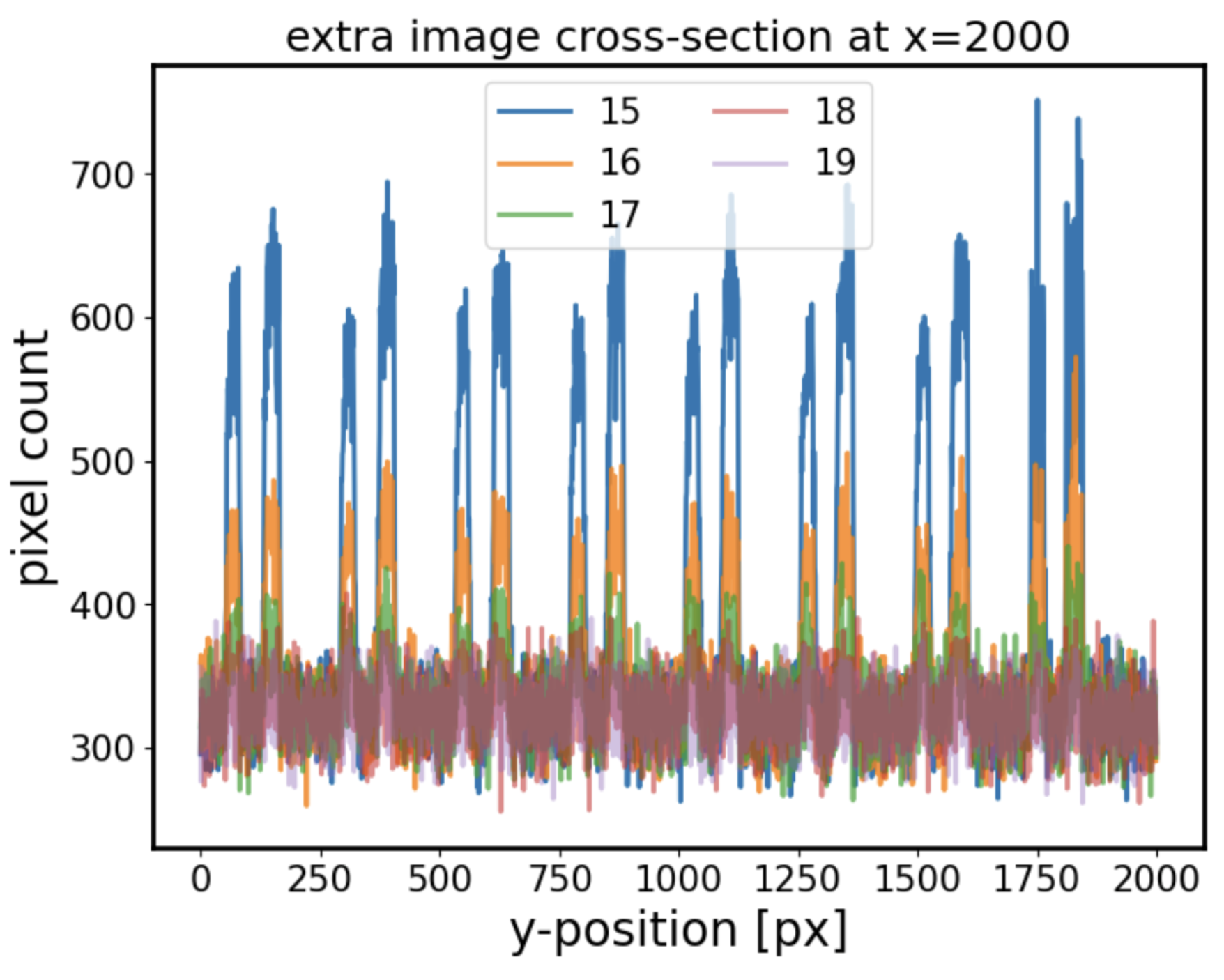
For example images below show backgroundmode 0 grids of stars of 15th magnitude: 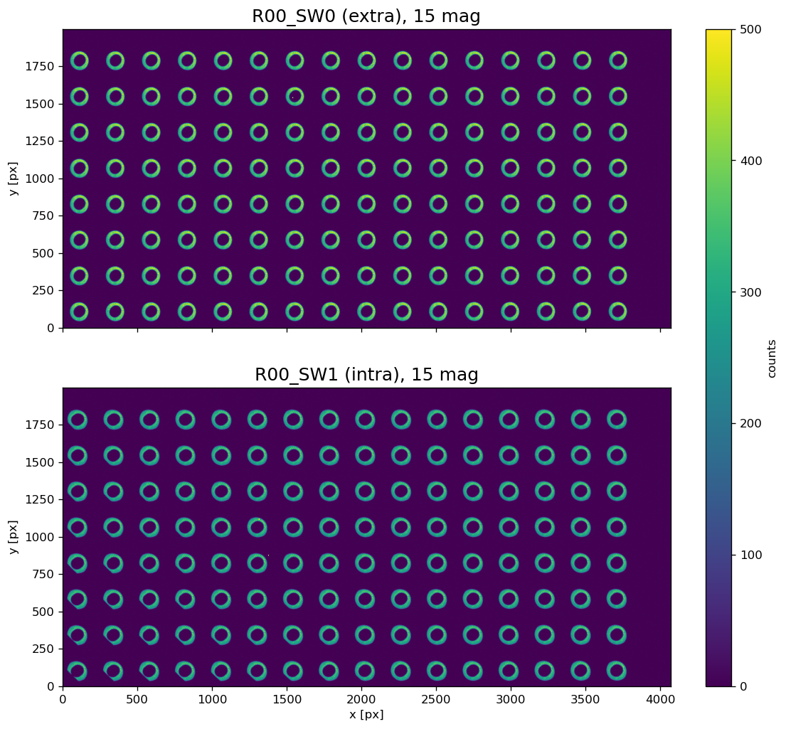
and 17th magnitude:
Simulating the OPD
The Optical Path Difference (OPD) is the difference between idealized reference sphere wavefront vs real aberrated wavefront. The OPD returned by phoSim assumes knowledge of the mirror shape, including any perturbations to their surface. By default for the corner wavefront sensors it is evaluated at 4 corners, at mid-point between each sensors. This makes sense as the reference OPD since the average location of all sources taken from each half-sensor would be somewhere in between the two sensors
if sources are distributed uniformly. However, to ensure that the differences of estimated wavefront are not due to intrinsic differences of the OPD at different locations, we need to evaluate the OPD at source locations. Thus we use exactly the same perturbation cmd files as when simulating the stellar grid, but we alter the inst files, outputing images to iter0/img/opd_grid/ sub-directory.
We modify an example phosim call from imgCloseLoop log:
INFO:PHOSIM OPD ARGSTRING: /sdf/data/rubin/u/scichris/WORK/AOS/DM-36218/wfs_grid_18/iter0/pert/opd.inst -i lsst -e 1 -c /sdf/data/rubin/u/scichris/WORK/AOS/DM-36218/wfs_grid_18/iter0/pert/opd.cmd -p 300 -o /sdf/data/rubin/u/scichris/WORK/AOS/DM-36218/wfs_grid_18/iter0/img -w /sdf/data/rubin/u/scichris/WORK/AOS/DM-36218/wfs_grid_18/iter0/img > /sdf/data/rubin/u/scichris/WORK/AOS/DM-36218/wfs_grid_18/iter0/img/opdPhoSim.log 2>&1
to use different inst file, and output images to a different location:
python /sdf/group/rubin/ncsa-home/home/scichris/aos/phosim_syseng4/phosim.py /sdf/data/rubin/u/scichris/WORK/AOS/DM-36218/opd_grid.inst -i lsst -e 1 -c /sdf/data/rubin/u/scichris/WORK/AOS/DM-36218/wfs_grid_19/iter0/pert/opd.cmd -p 256 -o /sdf/data/rubin/u/scichris/WORK/AOS/DM-36218/wfs_grid_19/iter0/img/opd_grid/ -w /sdf/data/rubin/u/scichris/WORK/AOS/DM-36218/wfs_grid_19/iter0/img/opd_grid/ > /sdf/data/rubin/u/scichris/WORK/AOS/DM-36218/wfs_grid_19/iter0/img/opdPhoSimGrid.log 2>&1
Note that by default a simulation seed is the same in each run (governed by simSeed), so each run of imgCloseLoop that has the same starting parameters (eg. default) starts with exactly the same perturbations. This means that during separate runs of imgCloseLoop simulating different magnitudes of grid sources, we have exactly the same OPD. For this reason
in illustrations below we only show one grid of OPD values, which is the same for all magnitudes of sources.
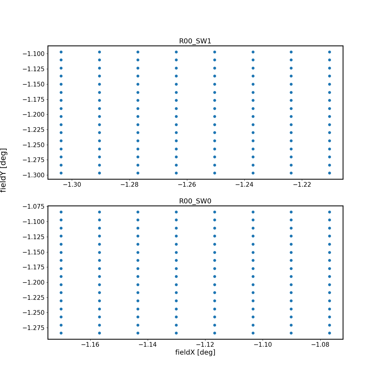
This figure illustrates location at which the OPD was evaluated:
Variation of the OPD
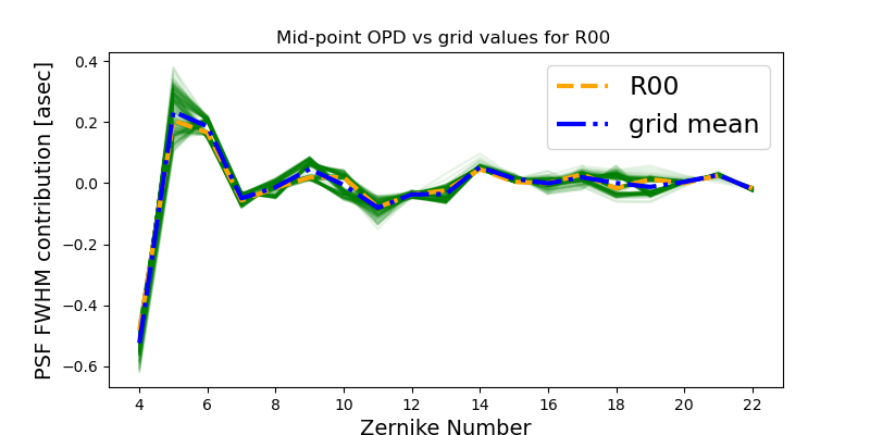
There is an intrinsic variation of the OPD that corresponds to variation of the wavefront at different points in the focal plane. This figure shows that the mean of the OPD evaluated at grid locations is very similar to the mid-point OPD evaluated by phosim, as we would expect from symmetry:
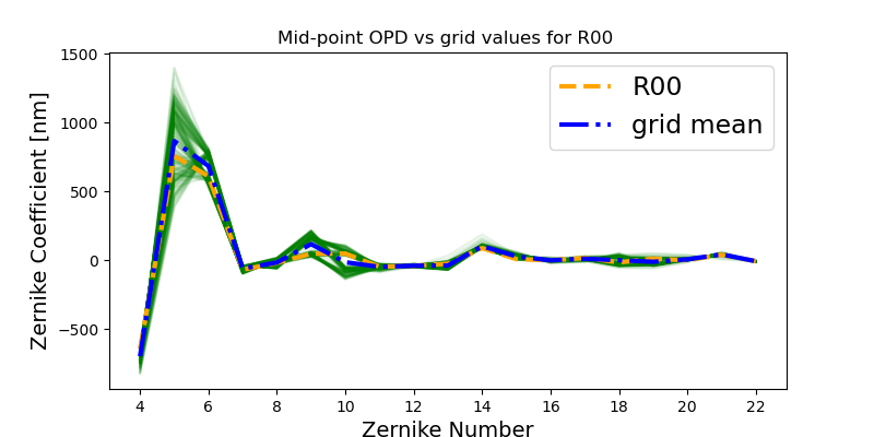
The difference between the mid-point OPD used in AOS calculations (orange) and the mean of grid OPD (blue) is on 1% level. Below the same is converted to PSF FWHM contribution with lsst.ts.phosim.utils.convertZernikesToPsfWidth . We plot the \(q_{OPD}\):
To quantify the magnitude of difference between OPD values at different points of the grid we calculate the RMS difference:
\(\Delta_{\mathrm{RMS}} = \sqrt{ \sum{|\mathrm{opd}_{i} - \left<\mathrm{opd}\right>|^{2}} / N}\)
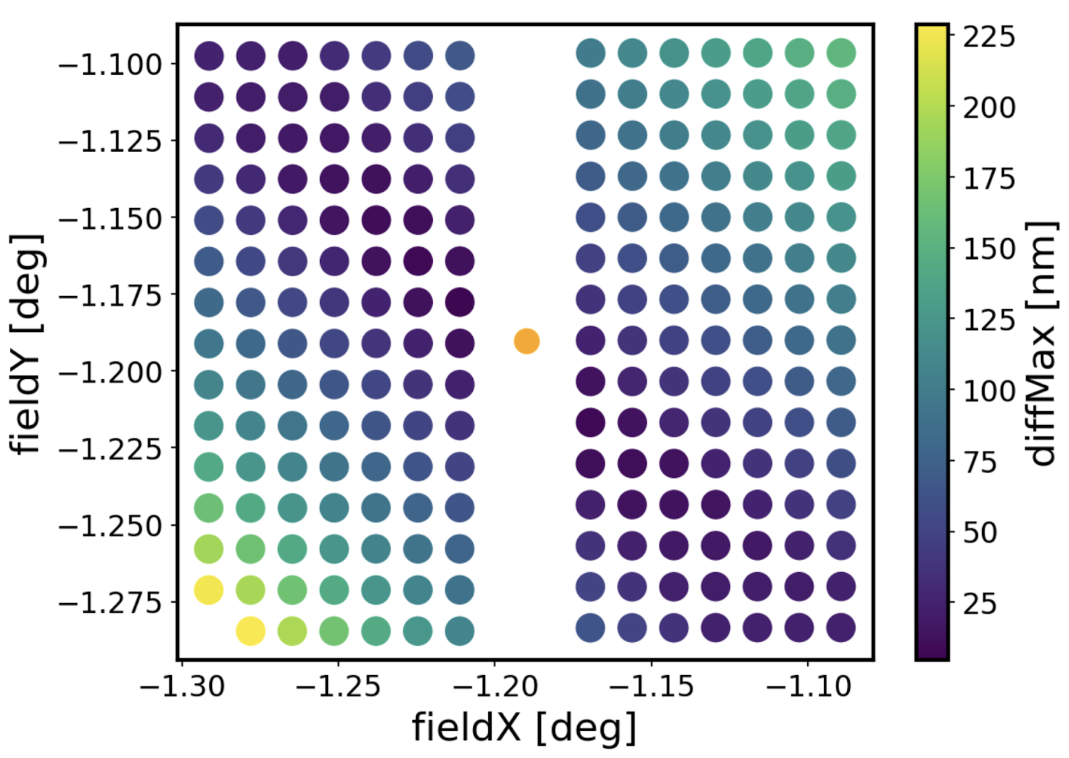
and the maximum difference:
\(\Delta_{\mathrm{MAX}} = \mathrm{max}(\mathrm{opd}_{i}-\left<\mathrm{opd}\right>)\)
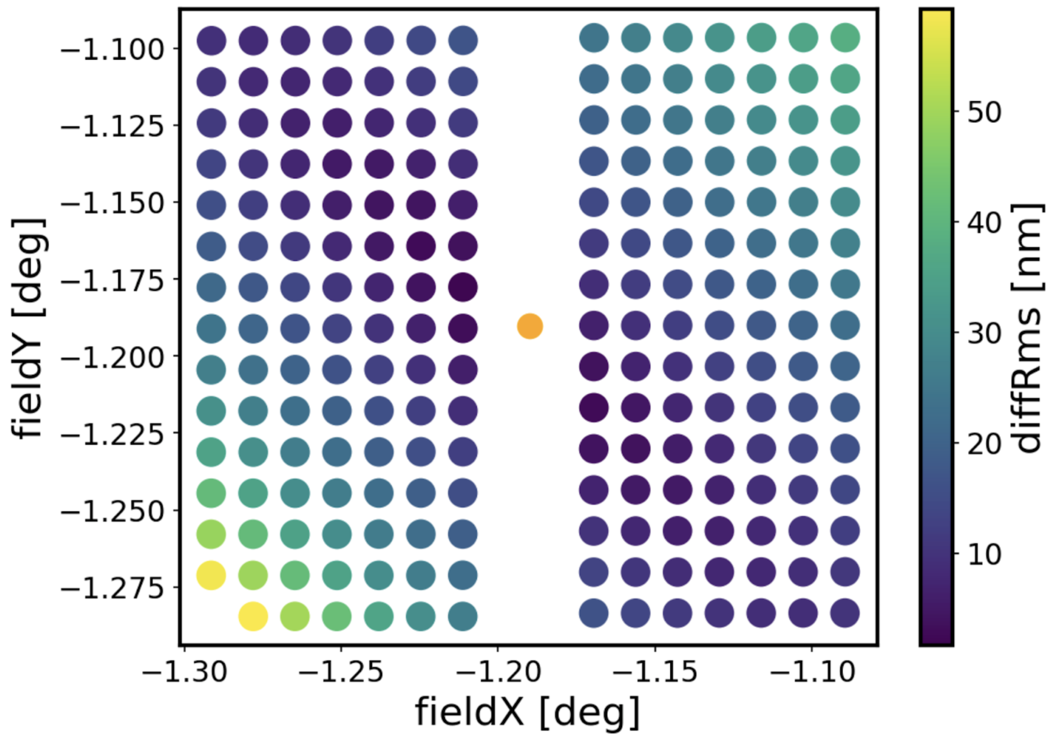
There’s a very small RMS difference (<20 nm) between the mean OPD and points at similar field radius. This suggests that there is an inherent structure to the OPD that is most dependent on the distance from the center of the field of view (OPD at similar fieldR have similar Zernikes, and those that have very different fieldR have much larger difference in their Zernikes).
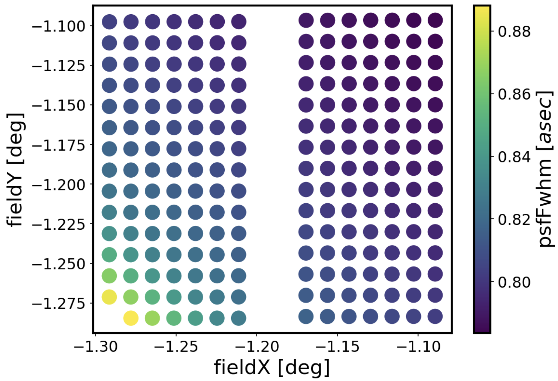
The OPD from nanometers can be converted to PSF FWHM contribution:
PSF FWHM [asec] = \(\sqrt{\sum_{i} q_{OPD,i}^{2}}\)
Numbering donuts
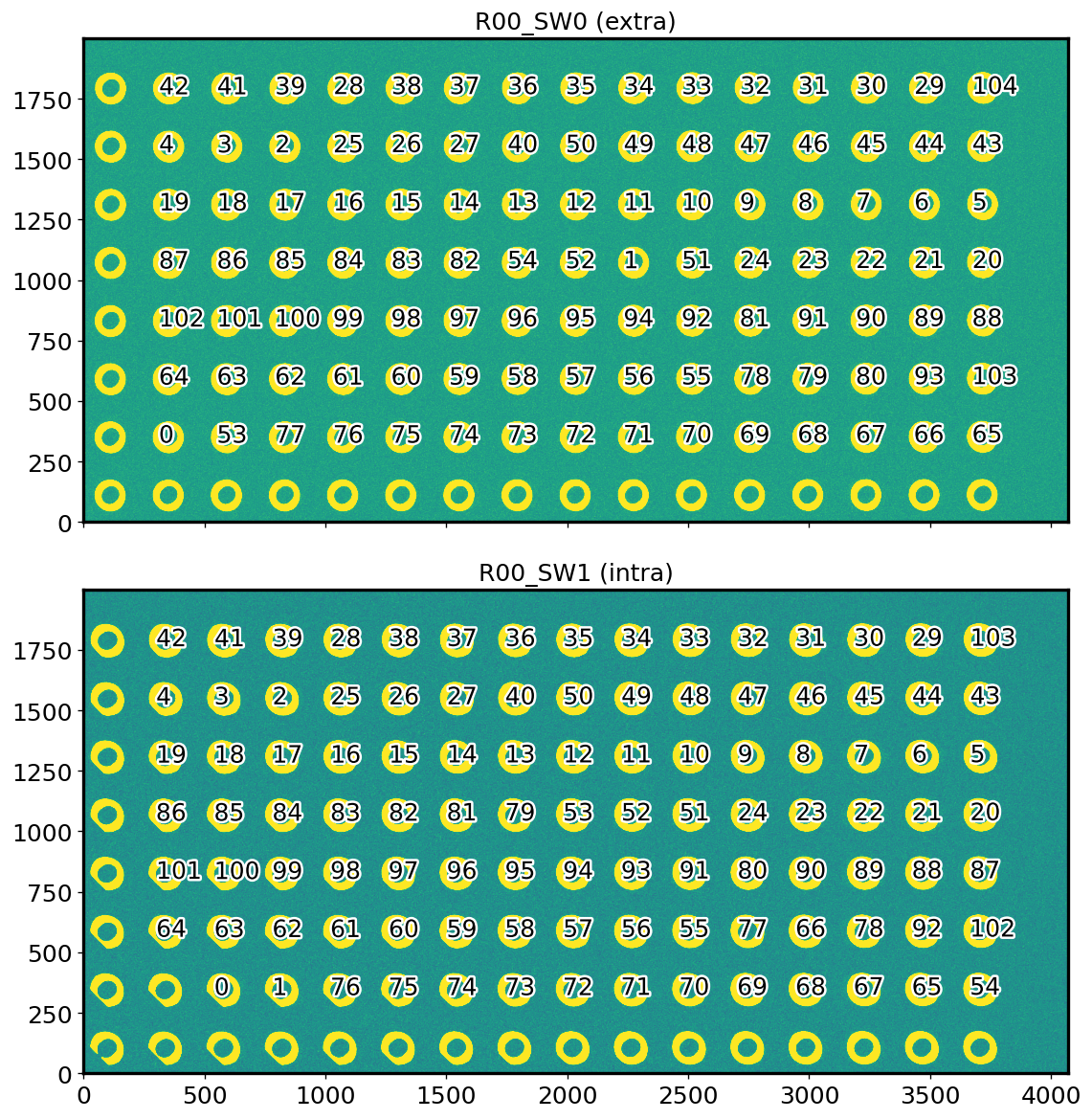
Currently the stars are paired up in ts_wep without eg. any selection for strength of vignetting. Below we put the index number in the donutStampsIntra, donutStampsExtra (corresponding to pair number passed to algorithm) showing that the pairing up of donuts does not follow any particular fashion other than the detection order:
Making A/B groups
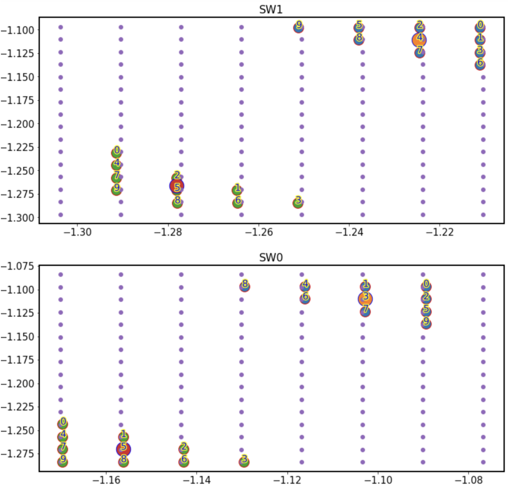
We perform stacking by creating two groups: A, which is in the least-vignetted corner, and B, in the most vignetted corner. We make the groups by sorting all donuts according to the field distance, and choosing twenty with the smallest, and same number of donuts with the largest field distance. The plot below illustrates locations of donuts in each group atop the OPD grid locations. Big red and orange dots mark the mean field X and Y position of all donuts within each group. For evaluating the wavefront for stacked donuts, we use that mean field location for donut mask evaluation.
Donut stacking
The imgCloseLoop simulation was run in each setup of source magnitude / brightness for several iterations to allow convergence tests. However, for all stacking tests we used donut stamps from the first iteration only.
Stacking was performed by selecting all donut stamp images within a given group. We define a stacked donut as a new donut where array count values correspond to a mean of all pixel values for a given (x,y) pixel location from all donuts stacked on top of each other. The field position of the stacked donut is the mean of all field(x,y) positions of donuts within a group (see large red and orange dots on a plot illustrating donut grouping).
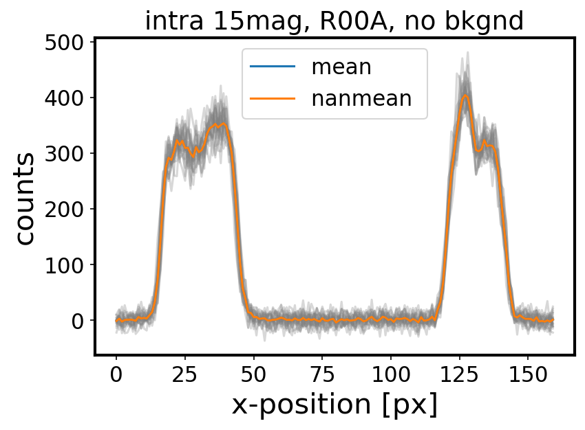
Two approaches to stacking : taking a numpy.mean vs numpy.nanmean are illustrated below. Since they yield close to identical results, with almost no nan pixels, we used a regular mean throughout.
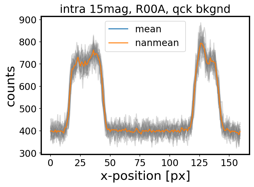
The addition of quick background does not change the donut cross-section shape, but does increase the counts by the background level (~300 counts for single exposure time):
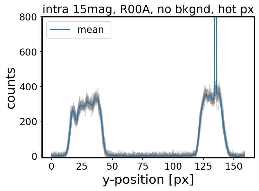
A small percentage of donut stamps was affected by a hot pixel - a pixel with an anomalously large value. For instance, for R00 sensor, this affected 2 out of 104 simulated donuts in the simulation with no background, using 15th mag sources. It was found that since this would drive the mean of the pixel values unnecessarily high at a position of hot pixel, these donuts were discarded and not included in groups A or B:
Comparing stacking within groups
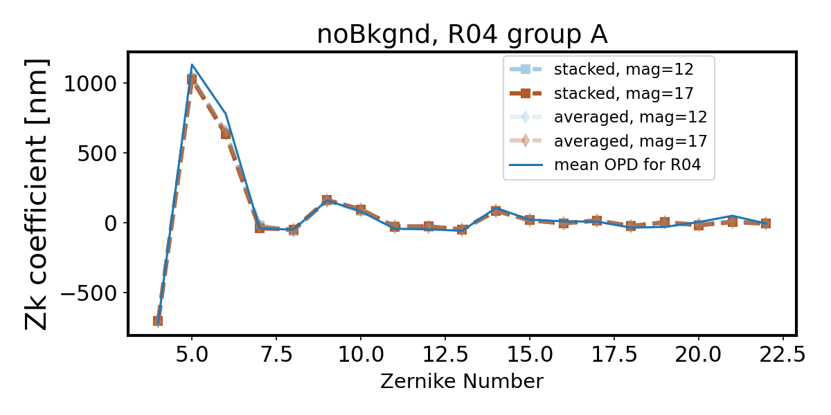
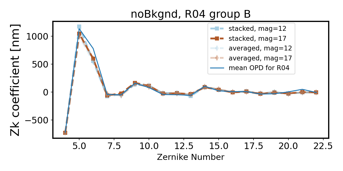
First we illustrate the variance of individual Zernike estimates from 20 donut pairs in group B in sensor R44. We plot the direct results of fitting, overplotting the average, and the result of stacking the donut postage stamp and performing a single fit 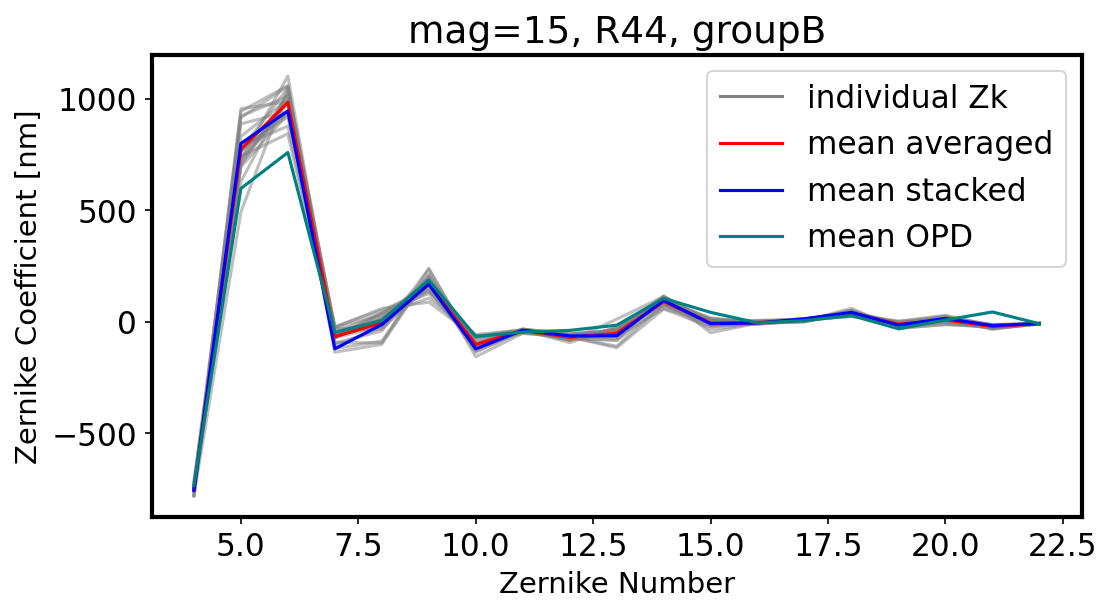
Here we illustrate the scatter, measured by the standard deviation, for all individual Zernike mode values per sensor group:
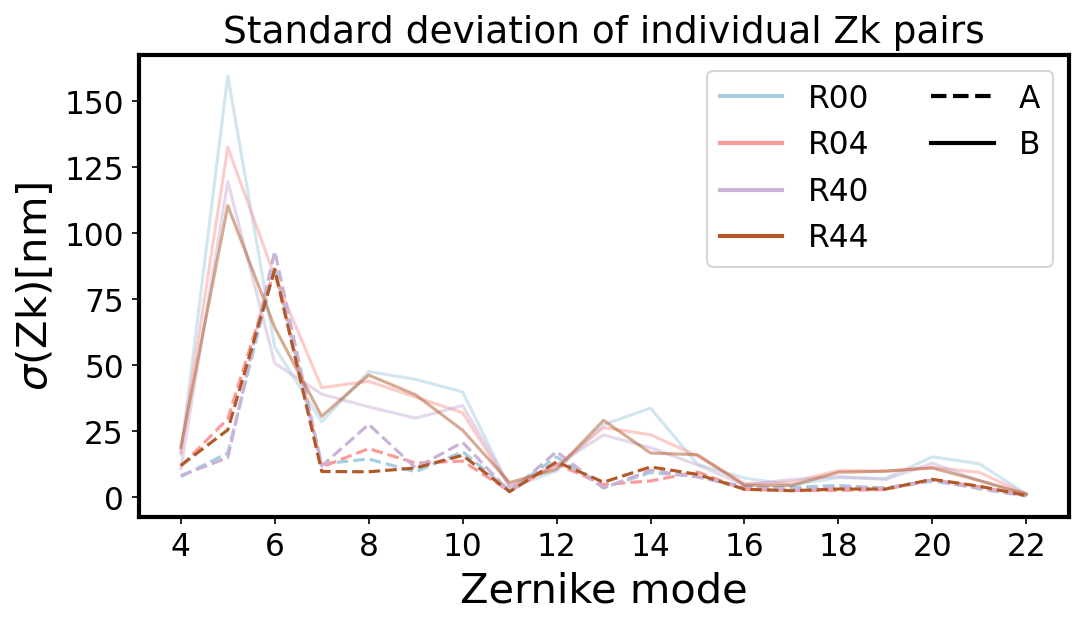
Within each group there is little dependence on magnitude for no simulated background. We notice that consistently group A (less vignetted) has a smaller departure from the OPD than group B (more vignetted), and the difference between stacking and averaging is harder to notice.
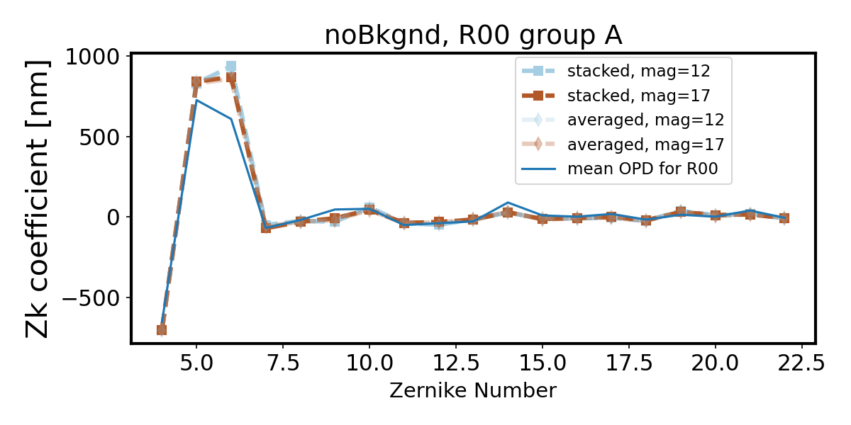
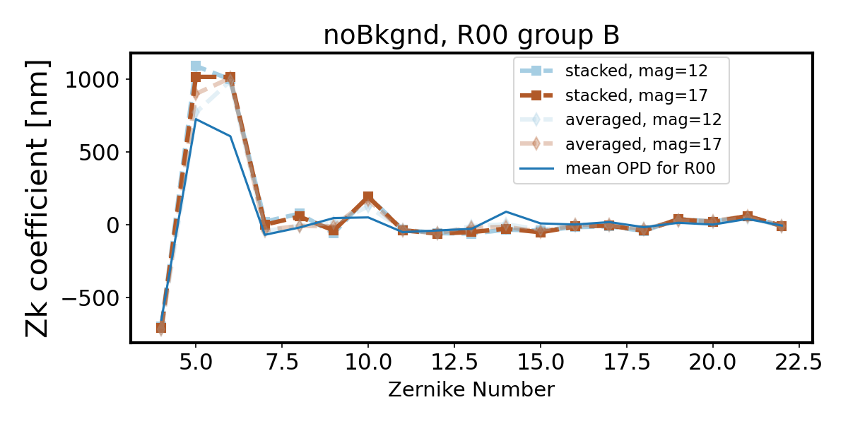
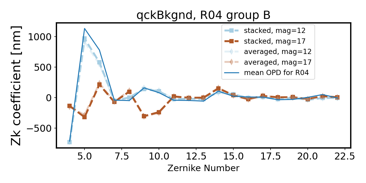
Introduction of quick background makes the wavefront recovery more difficult - we see degradation of Zernike estimate departing further from the OPD as the source brightness decreases (source magnitude increases). First we show only two magnitudes - note that while bright sources result in a fit very close to the OPD, faint sources (mag=17) are not well fit.
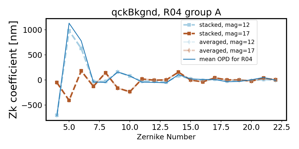
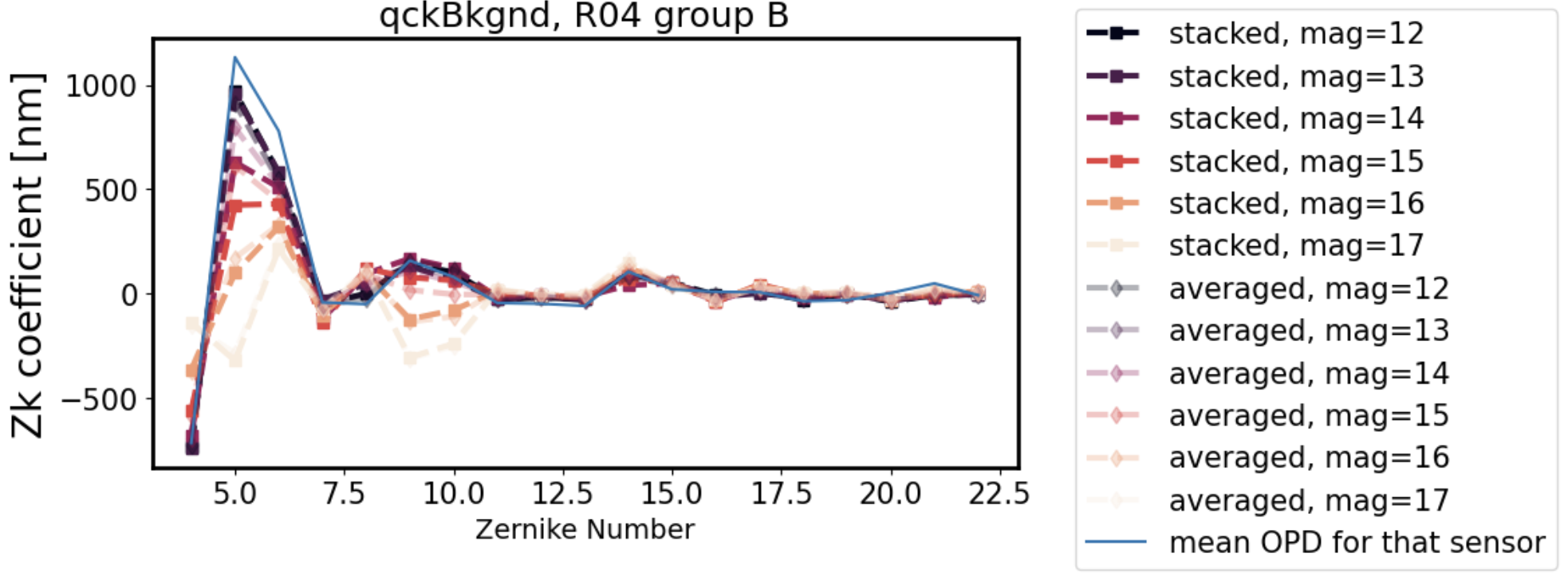
The following plots show that the degradation in fit fidelity from magnitude 12 to 17 is continuous, i.e. the fit degrades further and further away from the OPD the larger the source magnitude (lower the source brightness). All magnitudes are included for the same two sensors in this pair of plots: 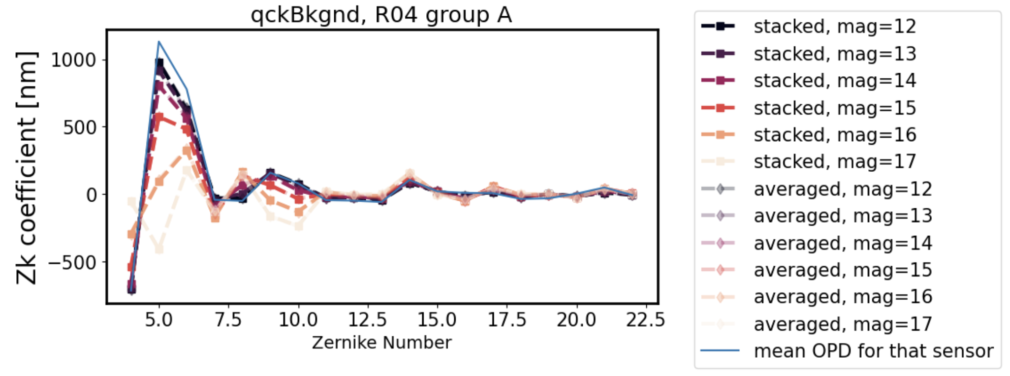
We can express that as a single metric per image : a PSF FWHM degradation. With
\(q_{OPD} = \mathrm{ConvertZernikesToPsfWidth}(Zk_{OPD})\), and
\(q_{EST} = \mathrm{ConvertZernikesToPsfWidth}(Zk_{estimated})\),
then contribution of the AOS to the PSF is \(\sqrt{(\sum_{i}{(q_{OPD,i}-q_{EST,i})^{2} })}\)
Thus we have a single number: the contribution to the PSF degradation due to an error in the AOS estimation (the difference between the OPD and the Zernike estimate) in arcseconds: PSF FWHM, per corner pair, per magnitude.
Plotting both groups on the same graph for a single corner, eg. R00 below, we see that the faint lines (B group, more vignetted) have higher degradation (on the level of 0.4-0.5 arcsec)
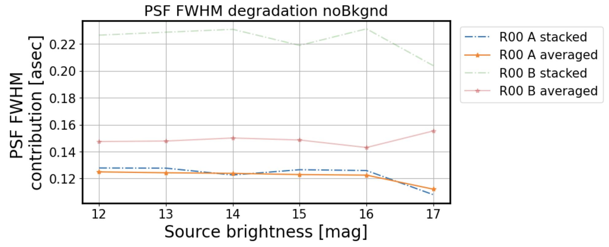
This is true for all simulations with no background - whether stacked or averaged , group B (faint dashed or solid lines) performs worse than group A (strong dashed or solid lines) - it has a higher PSF degradation:
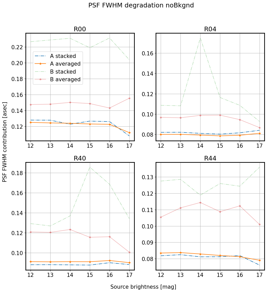
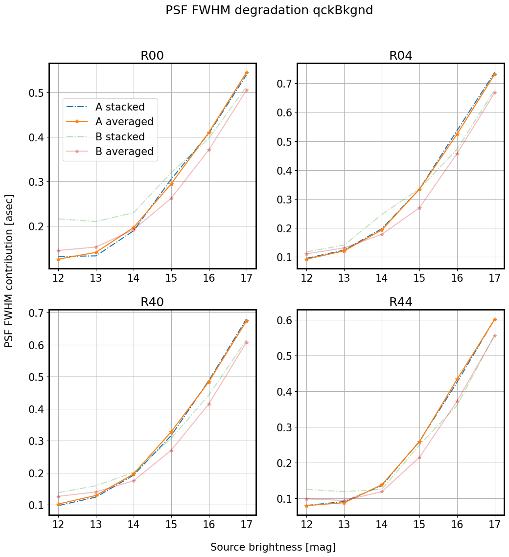
Thus whether stacked (dash-dot) or averaged (solid) , the main discriminant is the amount of vignetting. When we add background, the trend of increasing PSF degradation as a function of source magnitude becomes clear:
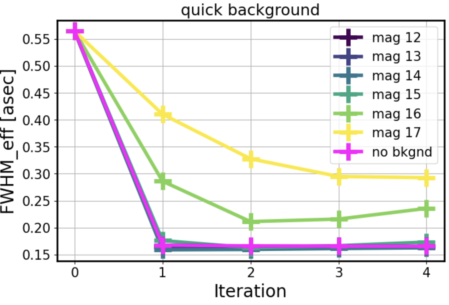
Impact of quickbackground on convergence of the AOS loop
We find that adding background to imgCloseLoop simulation with a stellar grid makes the AOS loop converge more slowly as the intensity of donuts gets closer to that of the background. Indeed, this is because as the source magnitude decreases, the intensity of a donut approaches that of the background:
Summary
In summary we performed a series of tests simulating stellar grid on corner sensors consisting of well separated sources of a single magnitude, with or without background. All simulations were allowed to run via imgCloseLoop for the default (5) iterations. We sorted donuts detected at 0th iteration for each intra- and extra-focal sensor by the distance from the center of the field. Of 105 donuts in each sensor, we select 20 nearest to the center of the field into group A, and those 20
farthest away from the center of the field (with highest vignetting) into group B. For each group we stack the donuts, and perform wavefront estimation on such single stacked donut. We also take individual donut pairs from each group, and fit these with ts_wep to obtain individual wavefront estimates that were averaged per each group. Thus for each corner sensor and group we compared the averaged to stacked Zernike estimates. We also simulated the optical path difference (OPD), that
represents the “truth” of the optical system, at the same grid points as the sources. We found that the mean of the OPD at the grid points to the OPD is within few nm to the OPD evaluated at the mid-point between the intra and extra-focal corner sensors (the OPD usually used in the AOS loop). We also tested the gradient in the OPD across the entire source grid, and found it to be <0.05 asec FWHM, i.e. smaller than the difference between group A and B, regardless of whether stacked or averaged.
We found that with no background there is no magnitude dependence, and the main difference in fit is between different corners and the amount of vignetting. We recommend to maintain the default strategy for wavefront estimation, i.e. averaging individual donut estimates, since we do not find evidence that stacking would perform better (with or without background).